
고정 헤더 영역
상세 컨텐츠
본문

작성자 : 14기 임혜리
참고 커널 : https://www.kaggle.com/chanoncharuchinda/top-100-korean-dramas
Top 100 Korean Dramas
Explore and run machine learning code with Kaggle Notebooks | Using data from Top 100 Korean Drama (MyDramaList)
www.kaggle.com
데이터 설명
top100_kdrama.csv 는 'MyDramaList'라는 외국 웹사이트에서 공개한 '한국 드라마 Top 100' 데이터이다.
beautifulsoup이라는 라이브러리를 통해 웹 크롤링을 진행하였다.
beautifulsoup : 인터넷 문서의 구조에서 명확한 데이터를 추출하고 처리하는 가장 쉬운 라이브러리
변수 설명
Name: Korean drama name
Year of release: Release year of the drama
Aired Date: Aired Date (start) - (end)
Aired On: Aired on what day(s) of the week
Number of Episode: How many episodes are there
Network: What Network is the drama aired on
Duration: How long is one episode approximately
Content Rating: Content raet for appropirate audience
Synopsis: Short story of the drama
Genre: Genre that the drama is listed in
Tags: Tags that the drama is listed in
Rank: Ranking on the website
Rating: Rating by the users on the website out of ten
라이브러리 설치
import pandas as pd
import numpy as np

import matplotlib.pyplot as plt
import seaborn as sns

import plotly.express as px
from plotly.offline import init_notebook_mode, iplot
import plotly.graph_objects as go
init_notebook_mode(connected=True)

import warnings
warnings.filterwarnings("ignore")
데이터 불러오기
kdrama = pd.read_csv('top100_kdrama.csv')
kdrama.head()
데이터를 불러온 후, head 메서드로 데이터의 상단 부분을 확인한다.
kdrama.info()info 함수를 통해 데이터에 대한 전반적인 정보를 확인한다
kdrama.isna().sum()결측치를 확인해보니 결측치가 없음을 확인할 수 있다.
kdrama.columns
데이터의 컬럼명도 확인해준다.
Released year and aired on
kdrama.groupby('Year of release').size().reset_index().rename(columns = {0:'Count'})

fig = px.bar(data_frame = kdrama.groupby('Year of release').size().reset_index().rename(columns = {0:'Count'}),
              x = 'Year of release',
              y = 'Count')

colors = ['DarkSalmon'] * 12
colors[-2] = 'DarkSeaGreen'
colors [-3], colors[-5] = 'MediumOrchid','MediumOrchid'

fig.update_traces(marker_color = colors)

fig.update_layout(title = {'text':'Korean Drama released by year',
                           'font_size':20},
                  font = dict(family = "Driod Sans Mono, monospace",
                              size = 15,
                              color = 'black'))

fig.show()
groupby() 연산자는 다양한 변수를 가진 데이터셋을 분석하는데 있어 매우 유용하다.
이는 집단, 그룹별로 데이터를 집계하거나 요약하는 것을 가능하게 한다.
여기서는 'Year of release'로 groupby 하였다.
Top100 kdrama에서는 2020년에 출시된 드라마가 20개로 가장 많은 비중을 차지하고 있음을 확인할 수 있다.
fig = px.bar(data_frame = kdrama.groupby(['Year of release','Aired On']).size().reset_index().rename(columns = {0:'Count'}),
             x = 'Year of release',
             y = 'Count',
             color = 'Aired On',
             barmode = 'stack',
             color_discrete_sequence=px.colors.qualitative.Pastel)

fig.update_layout(title = {'text':'Korean Drama relased by Year and Aired On',
                           'y' : 0.95,
                           'x' : 0.45,
                           'xanchor' : 'center',
                           'yanchor' : 'top',
                           'font_family': 'Gravity One, monospace',
                           'font_color' :'black',
                           'font_size': 20},
                  legend_title = 'Aired On (day of week)',
                  font = dict(family = 'Courier New, monospace',
                              size = 15,
                              color = 'midnightblue'
                  ))

fig.show()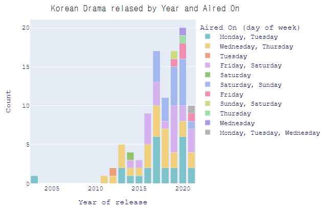
'Year of release', 'Aired On' 으로 groupby하게 되면 세부적인 정보를 얻을 수 있게 된다.
color 를 'Aired On'으로 지정하여 연도 내에서 무슨 요일에 하는 드라마가 더 높은 빈도를 차지 하고 있는지 확인해볼 수 있다.
Number of episodes
num_episode = kdrama['Number of Episode'].value_counts().reset_index().rename(columns={'Number of Episode':'Count','index':'Num Ep'})

# num_episode['Num Ep'] = num_episode['Num Ep'].apply(lambda s: f"#ep {s}")

fig = px.pie(data_frame = num_episode,
             values = 'Count', names = 'Num Ep',
             color_discrete_sequence = px.colors.qualitative.Safe)

fig.update_traces(textposition = 'inside',
                  textinfo = 'label+percent',
                  pull = [0.05] * num_episode['Num Ep'].nunique(),
                  insidetextorientation='horizontal')

fig.update_layout(title = 'Distribution of Number of Episodes among Top 100',
                  legend_title = 'Number of Episode',
                  uniformtext_minsize = 13,
                  uniformtext_mode = 'hide',
                  font = dict(family = 'Courier New, monospace',
                              size = 15,
                              color = 'black')
                  )

fig.show()
'number of episodes'를 기준으로 value_count를 한 후 pie chart로 표현한 것이다.
16부작 드라마가 43%로 가장 많은 비중을 차지하고 있음을 확인할 수 있다.
fig = px.bar(data_frame = num_episode,
             x = 'Num Ep', y = 'Count',
             title = 'Number of Episode Distribution')

fig.update_layout(xaxis_title = 'Number of Episode')

fig.update_xaxes(type='category')

fig.show()
Network
kdrama['Network'].value_counts()
'Network' 변수의 경우 어떤 네트워크를 통해 드라마가 방영되는지를 나타내고 있으므로 몇 가지 네트워크가 겹쳐서 나타나고 있음을 확인할 수 있다.
# This is NOT the most efficient way of doing this feature modification
# Since there aren't many unique value, this method (possibly) quickest and easiest to understand

def unique_network(networks):
    if networks == 'Netflix,  Netflix,  Netflix,  Netflix ':
        return 'Netflix'
    elif networks == 'tvN,  Netflix,  Netflix,  Netflix,  Netflix ':
        return 'Netflix, tvN'
    elif networks == 'OCN,  Netflix,  Netflix,  Netflix,  Netflix ':
        return 'Netflix, OCN'
    elif networks == 'jTBC,  Netflix,  Netflix,  Netflix,  Netflix ':
        return 'Netflix, jTBC'
    elif networks == 'KBS2,  Netflix,  Netflix,  Netflix,  Netflix ':
        return 'Netflix, KNS2'
    elif networks == 'SBS,  Netflix,  Netflix,  Netflix,  Netflix ':
        return 'Netflix, SBS'
    elif networks == 'Daum Kakao TV,  Netflix,  Netflix,  Netflix,  Netflix ':
        return 'Netflix, Daum Kakao TV'
    else:
        return networks

kdrama['Network'] = kdrama['Network'].apply(lambda networks: unique_network(networks))
kdrama['Network'].value_counts()
unique한 값으로 만들어주기 위해 조건문을 포함하고 있는 unique_network라는 함수를 지정해줬다.
feature modification에서 가장 효과적인 방법은 아니지만 빠르고 쉽게 이해시키기 위해 위 방법을 사용했다고 커널에 나와있다.
# Counting individual network
from collections import Counter

network_list = []
for networks in kdrama['Network'].to_list():
    networks = networks.strip().split(", ")
    for network in networks:
        network_list.append(network)

network_df = pd.DataFrame.from_dict(Counter(network_list),orient='index').rename(columns={0:'Count'})
network_df.sort_values(by='Count',ascending = False,inplace = True)
network_df
unique한 값들로 구분되어 빈도를 나타내고 있음을 확인할 수 있다.
네트워크의 경우 tvN 그리고 Netflix 순으로 높은 빈도를 보이고 있다.
fig = px.bar(data_frame = network_df,
             x = network_df.index,
             y = 'Count')

fig.update_layout(title = "Distribution of Korean Drama on different Networks",
                  xaxis_title = 'Network')

fig.show()
fig = px.pie(data_frame = network_df,
             values = 'Count',
             names = network_df.index,
             color_discrete_sequence = px.colors.qualitative.Prism)

fig.update_traces(textposition ='inside',
                  textinfo = 'label+percent',
                  pull = [0.05] * len(network_df.index.to_list()),
                  insidetextorientation='horizontal')

fig.update_layout(paper_bgcolor = 'white',
                  title = 'Network Distribution',
                  legend_title = 'Network',
                  uniformtext_minsize=18,
                  uniformtext_mode='hide',
                  font = dict(
                      family = "Courier New, monospace",
                      size = 18,
                      color = 'black'
                  ))

fig.show()
Duration of each episode
duration_df = kdrama['Duration'].value_counts().reset_index().rename(columns = {'Duration':'Count','index':'Duration'})

fig = px.bar(data_frame = duration_df.head(10),
             x = 'Duration',
             y = 'Count')

fig.update_layout(title = 'Kdrama Duration Distribution')

fig.show()
한 에피소드 당 소요되는 시간을 살펴보면 60분을 기준으로 하는 드라마가 가장 많음을 확인할 수 있다.
Content Rating
fig = px.bar(data_frame = kdrama['Content Rating'].value_counts().reset_index().rename(columns = {'Content Rating':'Count','index':'Con. Rate'}),
             x = 'Con. Rate',
             y = 'Count')

fig.show()
content rating은 대한민국의 영상물 등급 제도를 의미한다.
만 15세 이상 관람가 등급에 해당하는 드라마가 89개로 가장 많이 차지하고 있음을 확인할 수 있다.
# Content Rating by year
fig = px.bar(data_frame = kdrama.groupby(['Year of release','Content Rating']).size().reset_index().rename(columns = {0:'Count'}),
             x = 'Year of release',
             y = 'Count',
             color = 'Content Rating',
             barmode = 'stack',
             color_discrete_sequence=px.colors.qualitative.Pastel_r)

fig.update_layout(title = {'text':'Korean Drama relased by Year and Content Rating',
                           'y' : 0.95,
                           'x' : 0.45,
                           'xanchor' : 'center',
                           'yanchor' : 'top',
                           'font_family': 'Gravity One, monospace',
                           'font_color' :'black',
                           'font_size': 20},
                  legend_title = 'Content Rating',
                  font = dict(family = 'Courier New, monospace',
                              size = 15,
                              color = 'midnightblue'
                  ))

fig.show()
'Year of release', 'Content Rating' 변수를 기준으로 group_by를 진행하여 시각화한 것이다.
Top100 안에 위치한 드라마 중에서 2019, 2020년의 경우 19세 이상 관람가로 판정된 드라마가 각각 4개, 3개인 것을 확인할 수 있다.
Gneres and Tags
# Individual Genre
kdrama['Genre'] = kdrama['Genre'].str.strip()

genre_list = list()
for genres in kdrama['Genre'].to_list():
    genres = genres.split(",  ")
    for gen in genres:
        genre_list.append(gen)

genre_df = pd.DataFrame.from_dict(Counter(genre_list), orient = 'index').rename(columns = {0:'Count'})
genre_df.sort_values(by='Count',ascending = False, inplace = True)
genre_df.head()
fig = px.bar(data_frame = genre_df,
             x = genre_df.index,
             y = 'Count')

fig.update_layout(title = 'Genre Distribution',
                  xaxis_title = 'Genre')

fig.show()
장르로 구분해보면 드라마, 로맨스, 코미디 순으로 높은 빈도를 보인다.
# Individuals Tags
tags_list = list()

for tags in kdrama['Tags'].to_list():
    tags = tags.split(", ")
    for tag in tags:
        tags_list.append(tag)

tags_df = pd.DataFrame.from_dict(Counter(tags_list), orient = 'index').rename(columns = {0:'Count'})
tags_df.sort_values(by='Count',ascending = False, inplace = True)
tags_df.head()
fig = px.bar(data_frame = tags_df.head(10),
             x = tags_df.iloc[:10].index,
             y = 'Count')

fig.update_layout(title = 'Top 10 Tags Distribution',
                  xaxis_title = 'Tags')

fig.show()
드라마를 대표하는 Tag 단어로 구분해보면 'Strong Female Lead'로 태그된 드라마가 가장 많은 빈도를 보이고 있음을 확인할 수 있다.
Drama rating
# Max and Min Rating in the Top 100 Korean Drama
kdrama['Rating'].max(), kdrama['Rating'].min()
드라마 평가 점수의 최대와 최소를 구해보니 각각 9.2점과 8.5점임을 알 수 있다.
# Best Drama Rating
kdrama[kdrama['Rating'] == kdrama['Rating'].max()]
가장 높은 점수인 9.2점을 받은 드라마는 'Move to Heaven' 이었다.
kdrama[kdrama['Rating'] == kdrama['Rating'].min()].head()
8.5점을 받은 드라마 중 head메서드를 통해 무슨 드라마가 이에 속하는지 확인해볼 수 있다.
Actors and actresses in the drama
cast_list = list()

for casts in kdrama['Cast'].to_list():
    casts = casts.split(", ")
    for a in casts:
        cast_list.append(a)

cast_df = pd.DataFrame.from_dict(Counter(cast_list),orient = 'index').rename(columns = {0:'Appearance'})
cast_df.sort_values(by='Appearance',ascending = False,inplace = True)
cast_df.head()
Top100 순위권에 든 한국 드라마 중 송중기, 이준혁, 김지원 배우가 참여한 작품이 많다는 것을 확인할 수 있다.
Korean drama recommendation system
from sklearn.feature_extraction.text import CountVectorizer
from sklearn.metrics.pairwise import cosine_similarity

features = ['Duration','Synopsis','Cast','Genre','Tags']
kdrama['Number of Episode'] = kdrama['Number of Episode'].astype(str)

# kdrama['combined_features'] = kdrama['Duration'] + " " + kdrama['Synopsis'] + " " + kdrama['Cast'] + " " + kdrama['Genre'] + " " + kdrama['Tags'] + " " + kdrama['Number of Episode'] + " " + kdrama['Content Rating']

kdrama['combined_features'] = kdrama['Synopsis'] + " " + kdrama['Genre'] + " " + kdrama['Tags']

cv = CountVectorizer()
count_matrix = cv.fit_transform(kdrama['combined_features'])
cosine_sim = cosine_similarity(count_matrix)CountVectorizer는 문서 집합에서 단어 토큰을 생성하고 각 단어의 수를 세어 BOW 인코딩 벡터를 만든다.
BOW(Bag of Words)인코딩은 문서를 숫자 벡터로 변환하는 가장 기본적인 방법으로 전체 문서를 구성하는 고정된 단어장(vocabulary)를 만들고 개별 문서에 단어장에 해당하는 단어들이 포함되어 있는지를 표시하는 방법
문서 유사도란 문서와 문서 간의 유사도가 어느 정도인지 나타내는 척도로 그 방법 중 하나로 코사인 유사도(cosine_similarity)를 말 할 수 있다
Scikit-Learn의 문서 전처리 기능 — 데이터 사이언스 스쿨
.ipynb .pdf to have style consistency -->
datascienceschool.net
코사인유사도(Cosine similarity)란 벡터와 벡터 간의 유사도를 비교할 때 두 벡터간의 사잇각을 구해서 얼마나 유사한지 수치로 나타낸 것이다.

NLP - 8. 코사인 유사도(Cosine Similarity)
문서 유사도란 말그대로 문서와 문서 간의 유사도가 어느정도인지 나타내는 척도입니다. 문서 간 유사도를 측정해 지금 보고 있는 뉴스와 가장 유사한 뉴스를 추천해주기도 하고, 줄거리를 기
bkshin.tistory.com
'Number of Episode'의 데이터 타입을 astype()함수를 사용하여 문자열로 바꾸고 모든 변수에 대한 정보를 담는 'combined_features'열을 추가한다.
그 후 countervectorizer 라이브러리를 통해 벡터화된 행렬로 변환한 후 코사인 유사도를 담고 있는 오브젝트를 생성한다.
# Function for movie recommendation
def kdrama_recommendation(mov,sim_num = 5):

    user_choice = mov

    try:
        ref_index = kdrama[kdrama['Name'].str.contains(user_choice, case = False)].index[0]

        similar_movies = list(enumerate(cosine_sim[ref_index]))

        sorted_simmilar_movies = sorted(similar_movies, key = lambda x: x[1], reverse = True)[1:]

        print('\nRecomended K Drama for [{}]'.format(user_choice))
        print('-'*(24 + len(user_choice)))

        for i, element in enumerate(sorted_simmilar_movies):
            similar_movie_id = element[0]
            similar_movie_title = kdrama['Name'].iloc[similar_movie_id]
            s_score = element[1]
            print('{:40} -> {:.3f}'.format(similar_movie_title, s_score))

            if i > sim_num:
                break
    except IndexError:
        print("\n[{}] is not in our database!".format(user_choice))
        print("We couldn't recommend anyting...Sorry...")
# Search for movie with the keyword
def kdrama_available(key):
keyword = key
print("Movie with keyword: [{}]".format(keyword))
for i, mov in enumerate(kdrama[kdrama['Name'].str.contains(keyword)]['Name'].to_list()):
print("{}) {} ".format(i+1,mov))'kdrama_recommendation'과 'kdrama_available'이라는 함수를 생성한다
kdrama_available('It')
'kdrama_available'함수에 'It'을 입력하면 드라마 'Name'에 'It'을 포함하고 있는 드라마들이 무엇이 있는지 알 수 있다.
kdrama_recommendation("It's Okay to Not Be Okay")
'kdrama_recommendation'함수에 'It's Okay to Not Be Okay'를 입력하면 유사한 드라마의 'Name'과 cosine similarity 값을 확인해볼 수 있다.
from sklearn.feature_extraction.text import TfidfVectorizer
from sklearn.metrics.pairwise import linear_kernel

tfdif_vector = TfidfVectorizer(stop_words = 'english')

tfidf_matrix = tfdif_vector.fit_transform(kdrama['Synopsis'])

sim_matrix = linear_kernel(tfidf_matrix, tfidf_matrix)

indicies = pd.Series(kdrama.index, index = kdrama['Name']).drop_duplicates()
TF-IDF(Term Frequency-Inverse Document Frequency)인코딩은 단어를 갯수 그대로 카운트 하지 않고 모든 문서에 공통적으로 들어있는 단어의 경우 문서 구별 능력이 떨어진다고 보아 가중치를 축소하는 방법
CounterVectorizer와 비슷하지만 단어의 가중치를 조정한 후 BOW 인코딩 벡터를 만든다는 것이 차이점이다.
Stop Words는 문서에서 단어장을 생성할 때 무시할 수 있는 단어를 말한다. 보통 영어의 관사나 접속사, 한국어의 조사 등이 여기에 해당한다.
영어에서 stop words는 a, the, is, are 등을 말할 수 있다.
kernel이란 선형 분리가 불가능한 데이터에서 kernel function을 통해서 선형 분리가 가능한 새로운 높은 차원의 데이터로 변환시키는 방법, non_linear한 문제를 linear하게 transform 하여 더 쉽게 해결할 수 있도록 한다.
kdrama데이터의 'Synopsis' 열의 데이터를 대상으로 TF-IDF 인코딩을 진행한다.
def content_based_recommender(title, sim_scores = sim_matrix):
    idx = indicies[title]

    sim_scores = list(enumerate(sim_matrix[idx]))

    sim_scores = sorted(sim_scores, key = lambda x : x[1], reverse = True)

    sim_scores = sim_scores[1:11]

    drama_score = list()
    for score in sim_scores:
        drama_score.append(score[1])

    kdrama_indices = [i[0] for i in sim_scores]

    kdrama_name = kdrama['Name'].iloc[kdrama_indices]

    print('\nRecomended KDrama for [{}]'.format(title))
    print('-'*(24 + len(title)))
    for score,name in list(zip(drama_score,kdrama_name)):
        print("{:30} -> {:.3f}".format(name,score))
'content_based_recommer'라는 함수를 생성한다.
content_based_recommender("It's Okay to Not Be Okay")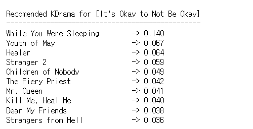
'content_based_recommender'함수에 'It's Okay to Not Be Okay'를 입력하면 'It's Okay yo Not Be Okay'의 Synopsis 즉 개요와 유사도가 높은 드라마의 'Name'과 점수를 확인할 수 있다.
# nltk
import nltk
nltk.download('punkt')
nltk.download('averaged_perceptron_tagger')
nltk.download('wordnet')
NLTK 라이브러리는 텍스트 분류, 토큰화, 단어 stemming, 품사 태킹, 텍스트 파싱, semantic reasoning 등을 하는데 사용하는 텍스트 자연어 처리 파이썬 모듈이다.
처음 사용하는 경우에는 nltk.downlodad('punkt')를 실행하여 Punket Tokenizer Models (13MB)를 다운로드 해주어야 한다.
nltk.download('averaged_perceptron_tagger')로 태깅에 필요한 자원을 다운로드 해주어야 토큰들에 대해서 품사 태킹을 할 수 있게 된다.
WordNet은 어휘에 중점을 둔 영어사전 Database이다. 약 16만개의 단어와 12만개의 유사어 집합을 포함하고 있는 방대한 thesaurus(시소러스, 유의어 사전)
https://rfriend.tistory.com/546
[Python] NLTK(Natural Language Toolkit)와 WordNet으로 자연어 처리하기 맛보기
이번 포스팅에서는 Python의 NLTK (Natural Language Toolkit) 라이브러리와 WordNet 말뭉치를 사용하여 자연어 처리 (Natural Language Processing) 하는 몇 가지 방법을 맛보기로 소개하겠습니다. (저는 Python..
rfriend.tistory.com
from nltk.stem import WordNetLemmatizer
lemmatizer = WordNetLemmatizer()

from nltk.corpus import stopwords
nltk.download('stopwords')
stop_words = set(stopwords.words('english'))

VERB_CODES = {'VB', 'VBD', 'VBG', 'VBN', 'VBP', 'VBZ'}
NLTK에서는 표제어 추출을 위한 도구인 WordNetLemmatizer를 지원한다. 표제어(Lemma)란 기본 사전형 단어 정도로 이해하면 된다. 예를 들어 am, are, is는 서로 다른 스펠링을 가지고 있지만 그 뿌리 단어는 be라고 볼 수 있고 이를 표제어로 말할 수 있다.
위에서 특정 품사 약어를 담은 dictionary를 생성했음을 알 수 있다.
VB는 verb, base form(take), VBD는 verb, past tense(took), VBG는 verb, present participle(taking), VBN은 verb, past participle(taken), VBP는 verb, sing.present, non-3d(take), VBZ는 verb, 3rd present sing.presnt(takes)를 의미한다.
def preprocess_sentences(text):
    text = text.lower()
    temp_sent =[]
    words = nltk.word_tokenize(text)
    tags = nltk.pos_tag(words)
    for i, word in enumerate(words):
        if tags[i][1] in VERB_CODES:
              lemmatized = lemmatizer.lemmatize(word, 'v')
        else:
              lemmatized = lemmatizer.lemmatize(word)
        if lemmatized not in stop_words and lemmatized.isalpha():
              temp_sent.append(lemmatized)

    finalsent = ' '.join(temp_sent)
    finalsent = finalsent.replace("n't", " not")
    finalsent = finalsent.replace("'m", " am")
    finalsent = finalsent.replace("'s", " is")
    finalsent = finalsent.replace("'re", " are")
    finalsent = finalsent.replace("'ll", " will")
    finalsent = finalsent.replace("'ve", " have")
    finalsent = finalsent.replace("'d", " would")
    return finalsent

kdrama_copy = kdrama.copy()
kdrama_copy['synopsis_processed'] = kdrama_copy['Synopsis'].apply(preprocess_sentences)
kdrama_copy['synopsis_processed'].head()
'preprocess_sentence'라는 함수를 생성한다.
셀을 확인해보면, 문장들을 전처리하는 과정을 볼 수 있다.
tfdifvec = TfidfVectorizer()
tfdif_drama_processed = tfdifvec.fit_transform((kdrama_copy['synopsis_processed']))

co_sin_drama = cosine_similarity(tfdif_drama_processed,tfdif_drama_processed)
# Storing indices of the data
indices = pd.Series(kdrama_copy['Name'])
def recommendations(title, cosine_sim = co_sin_drama):
recommended_movies = []
index = indices[indices == title].index[0]
similarity_scores = pd.Series(cosine_sim[index]).sort_values(ascending = False)
top_10_movies = list(similarity_scores.iloc[1:11].index)
for i in top_10_movies:
recommended_movies.append(list(kdrama_copy['Name'].index)[i])
for index in recommended_movies:
print(kdrama_copy.iloc[index]['Name'])'recommendations'라는 함수를 생성한다. 이 함수는 cosine_similarity를 기준으로 top10개의 영화 'Name'을 출력한다.
recommendations("It's Okay to Not Be Okay")
'recommendations' 함수에 'It's Okay to Not Be Okay'를 입력하면 전처리 과정을 거친 synopsis 데이터를 기준으로 코사인 유사도가 높은 10개의 드라마 제목이 출력되는 것을 볼 수 있다!!
모두 수고 많으셨습니다 ^_^
'심화 스터디 > 코드 분석 스터디' 카테고리의 다른 글
| [코드 분석 스터디] StyleCLIP 구현하기 (0) | 2021.11.24 |
|---|---|
| [코드 분석 스터디] Spooky Author Prediction_NLP tutorial (0) | 2021.11.14 |
| [코드 분석 스터디] Natural Language Processing : Bag of Words for IMDB movie review (0) | 2021.11.13 |
| [코드 분석 스터디] Segmentation : Sementic Segmentation - CARLA Image Road segmentation (1) | 2021.11.04 |
| [코드 분석 스터디] Time Series Regression - Predict Future Sales 커널 필사 (2) | 2021.10.01 |


댓글 영역